Wireless Data Generation Pipeline
DeepMIMO sits at the center of a three-phase workflow for generating large-scale, ray-tracing-derived wireless datasets. The diagram below shows the full pipeline; this page walks through each phase and step in detail.
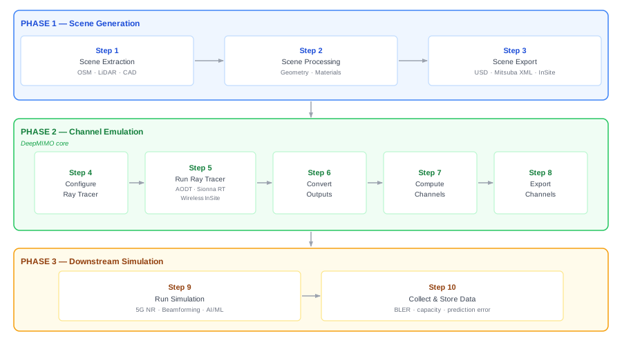
Phase 1 — Scene Generation
Phase 1 produces a 3D geometric scene that a ray tracer can consume. The inputs are real-world geographic data (GIS sources, OpenStreetMap, satellite imagery); the outputs are ray-tracer-specific scene files.
Step 1 — Scene Extraction
Fetch raw geometry from a GIS source. DeepMIMO's OSM pipeline queries OpenStreetMap via the Overpass API and returns building footprints, road networks, and terrain within a GPS bounding box.
from deepmimo.pipelines.blender_osm import fetch_osm_scene

fetch_osm_scene(
    minlat=40.752, minlon=-73.982,
    maxlat=40.756, maxlon=-73.977,
    output_folder="./times_square",
    output_formats=["insite", "sionna"],
)
Other GIS sources (LiDAR point clouds, urban digital twins, CAD files) can be used directly with the export step.
Step 2 — Scene Processing
Raw GIS data is often noisy or multi-source. This step merges, cleans, and normalizes the geometry:
- Trimming roads and buildings to the simulation bounding box
- Extruding 2D footprints into 3D building meshes
- Assigning material properties (concrete, glass, asphalt, …) to each surface
- Converting coordinates from GPS to Cartesian, storing the GPS origin for later reference
DeepMIMO's Blender pipeline handles this automatically when called with
fetch_osm_scene. For custom scenes, any mesh-editing tool (Blender, Open3D,
CGAL) can be used.
Step 3 — Scene Export
The processed scene is written to the native format of each target ray tracer.
| Ray Tracer | Format | Notes |
|---|---|---|
| NVIDIA AODT | OpenUSD (.usd / .usdc) |
Standard USD scene graph |
| Sionna RT | Mitsuba XML (.xml + meshes) |
Each surface as a Mitsuba shape |
| Remcom Wireless InSite | PLY buildings + .city / .ter files |
InSite-specific ASCII/binary formats |
The same bounding box and material assignments are written to all three formats simultaneously, ensuring that every ray tracer simulates the same physical environment.
Phase 2 — Channel Emulation
Phase 2 is DeepMIMO's core responsibility. It drives one or more ray tracers over a large number of TX/RX configurations and converts the outputs into a unified dataset format.
Step 4 — Configure Ray Tracer
This is the most complex step because every ray tracer exposes a different configuration API. DeepMIMO solves this in two complementary ways:
Option A — Ray-tracer-native configuration
Pass parameters directly to the target tracer (Sionna PathSolver kwargs,
InSite .setup XML fields, AODT config). Gives full control but requires
knowing each tracer's API.
Option B — DeepMIMO unified parameters
Define simulation parameters once using DeepMIMO's RTParams object. DeepMIMO
maps these to each tracer using a best-effort translation that preserves
physical equivalence as closely as the tracer allows:
rt_params = {
    "carrier_freq": 28e9,          # Hz
    "max_reflections": 5,
    "max_diffractions": 1,
    "max_scattering": 0,
    "max_transmissions": 2,        # InSite / AODT only
    "num_rays": 1_000_000,
    "synthetic_array": True,
}
| Parameter | AODT | Sionna RT | Wireless InSite |
|---|---|---|---|
| Carrier frequency | ✓ | ✓ | ✓ |
| Reflections | ✓ | ✓ | ✓ |
| Diffractions | ✓ | ✓ | ✓ |
| Transmissions | ✓ | ✗ (not supported) | ✓ |
| Diffuse scattering | ✓ | ✓ (final interaction only) | ✓ |
| Number of rays | ✓ | ✓ | ✓ |
| Synthetic array | ✓ | ✓ | ✓ |
Step 5 — Run Ray Tracer
DeepMIMO wraps each ray tracer with a thin pipeline layer that handles:
- Identical inputs — the same TX/RX positions and scene are fed to every tracer
- Batch processing — large RX grids are split into batches to fit GPU/RAM budgets
- Progress tracking —
tqdmbars show per-batch and per-TX-index progress - Output collection — paths are saved to disk in a tracer-agnostic intermediate format
# Sionna RT
from deepmimo.pipelines.sionna_rt import raytrace_sionna

raytrace_sionna(
    scene_path="./times_square/sionna_scene.xml",
    tx_pos=[[0, 0, 25]],
    rx_pos=rx_grid,
    save_folder="./rt_output/sionna",
    **rt_params,
)

# Wireless InSite
from deepmimo.pipelines.wireless_insite import raytrace_insite

raytrace_insite(
    osm_folder="./times_square",
    tx_pos=[[0, 0, 25]],
    rx_pos=rx_grid,
    save_folder="./rt_output/insite",
    wi_exe="/opt/insite/calcprop_server",
    wi_lic="/opt/insite/license.lic",
    **rt_params,
)
Automation difficulty varies by tracer:
| Tracer | Automation maturity |
|---|---|
| Sionna RT | Fully automated — pure Python API |
| NVIDIA AODT | Automated via USD + Python SDK |
| Remcom Wireless InSite | Automated via XML config + CLI launcher; requires InSite licence |
Step 6 — Convert Outputs
Raw ray-tracer outputs are parsed and converted into DeepMIMO's unified scenario
format (a set of .mat files per TX–RX pair, plus a params.json).
from deepmimo.converters import convert

convert("./rt_output/sionna", output_folder="./deepmimo_scenarios/times_square")
The converter normalizes path attributes (power, delay, angles, interaction types) across all three tracers so that downstream processing is tracer-agnostic. See Converters for format details.
Step 7 — Compute Channels
The converted ray-tracing data is loaded as a Dataset and channels are computed
for any antenna configuration and frequency plan:
import deepmimo as dm
from deepmimo.generator import ChannelParameters

ds = dm.load("times_square")
ch_params = ChannelParameters(
    bs_antenna={"shape": [8, 8]},
    ue_antenna={"shape": [1, 1]},
    ofdm={"num_subcarriers": 512, "bandwidth": 100e6},
)
ds.compute_channels(ch_params)
# ds["channel"] → [n_ue, M_rx, M_tx, K_subcarriers]
Step 8 — Export Channels
Computed channels are exported to whichever downstream format is required:
# Sionna upstream — feed channels back into Sionna PHY layer
from deepmimo.exporters import sionna_exporter
sionna_exporter(ds, output_folder="./sionna_input")

# AODT upstream
from deepmimo.exporters import aodt_exporter
aodt_exporter(ds, output_folder="./aodt_input")

# Raw numpy / pickle for custom use
ds.to_binary("./channels.pkl")
Phase 3 — Downstream Simulation
Phase 3 consumes the exported channels in an application-level simulator.
Step 9 — Run Simulation
The exported channel data drives the simulation block of interest. Examples:
- 5G NR link-level: compute BLER curves with realistic OFDM channels
- Beamforming: evaluate beam codebooks under spatially correlated channels
- Channel estimation: benchmark pilots, interpolation, and DNN estimators
- AI/ML training: feed channel sequences to prediction or classification models
DeepMIMO ships integration adapters for Sionna (PHY layer) so channels can be fed directly into Sionna's OFDM pipeline without manual reshaping.
Step 10 — Collect & Store Data
Simulation outputs (BLERs, capacity, prediction errors, …) are saved for analysis and, optionally, fed back into the DeepMIMO database to build a reproducible public dataset.
Related pages
- Pipelines capabilities — detailed feature matrix for each pipeline
- Comparing Ray Tracers — accuracy and performance comparison
- Ray Tracing Guidelines — parameter recommendations
- Converters — format details for each tracer's output
- Tutorials → Converters — end-to-end worked example